Machine Learning

Notes from Coursera.org/learn/machine-learning

Supervised Learning

Given the “right” answer for each training data

regression problem: predict real valued output
classification problem: discrete

Training Set Notation

$m$ : number of training examples – samples
$x$ : output variable – features
$y$ : output variable – target
$(x, y)$ : single example – sample
$(x^{(i)}, y^{(i)})$ : i-th training example

Training

ml training

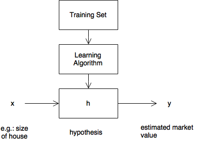
Hypothesis $h: {x}\rightarrow{y}$ produces estaimated value from features.

How is $h$ represented?

Linear Regression with One Variable

linear regression overview

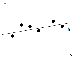
Linear regression function: $h_{\theta}(x)=\theta_{0}+\theta_{1}\cdot x$

Example Training Set

size (ft2) x	price ($1000) y
2104	460
1416	232
1539	315
852	178

hypothesis: $h_{\theta}(x)=\theta_{0}+\theta_{1}\cdot x$
parameters: $\theta_{i}$ -s

$\theta_{0}$	$\theta_{1}$	hypothesis
1	0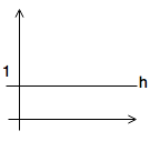
0	0.5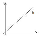
1	0.5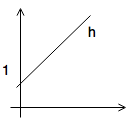

Cost Funtion

want: choose parameters $\theta_{0}$ and $\theta_{1}$ so that $h_{\theta}(x)$ is as close to $y$ for every training example as possible
want: minimize cost function $\min_{\theta_{0}, \theta_{1}} \frac{1}{2m}\sum_{i=1}^{m}{(h_{\theta}(x^{(i)})-y^{(i)})^2}$
cost function J is the squared error function we wish to minimize

$\begin{aligned} J(\theta_{0}, \theta_{1}) & = \frac{1}{2m}\sum_{i=1}^{m}{(h_{\theta}(x^{(i)})-y^{(i)})^2} \\ & = \frac{1}{2m}\sum_{i=1}^{m}{(\theta_{0} + \theta_{1}\cdot x^{(i)}-y^{(i)})^2}\end{aligned}$

squared error function is a good fit for most linear regressions problems

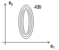
Gradient Descent

For minimizing the cost function.

Start with some $(\theta_{0},\theta_{1})$
Keep changing $\theta_{0}$ and $\theta{1}$ to reduce cost $J(\theta_{0},\theta_{1})$ unti we end up at a minimum
NB! Gradient descent generally applies to $J(\theta_{0},\theta_{1},...\theta_{n})$

Algorithm

start with say $(0,0)$
look around with a little step, take the direction which takes us the furthest down
repeat until convergence

NB! this takes us to a local optimum, not a global one

Pseudo Code

$\begin{aligned} & \text{repeat until convergence } \{ \\ & \qquad \theta_{j}:=\theta_{j}-\frac{\partial}{\partial\theta_{j}}\cdot\alpha\cdot\frac{1}{2m}\sum^{m}_{i=1}\Big(h_{\theta}(x^{(i)})-y^{(i)} \Big)^2 \quad\text{(for j=0..1)} \\ & \} \end{aligned}$

where $\alpha$ is the learning rate, ie.: the size of each step
adjusts each parameter with the resective partial derivative of the cost
NB! should update parameters simultaneously

Gradient Descent for Linear Regression

hypothesis: $h_{\theta}(x)=\theta_{0}+\theta_{1}\cdot x$
cost: $J(\theta)=\frac{1}{2m}\sum^{m}_{i=1}\big(h_{\theta}(x^{(i)})-y^{(i)} \big)^2$
gradient descent parameter update step: $\theta_{j}:=\theta_{j} - \alpha\cdot\frac{\partial}{\partial\theta_{j}}J(\theta)$

Partial Derivative of Cost Fn

NB! moving $\alpha$ learning rate outside of the partial derivative $\begin{aligned} & \frac{\partial}{\partial\theta_{j}}J(\theta_{0},\theta_{1}) & = & \frac{\partial}{\partial\theta_{j}}\frac{1}{2m}\sum^{m}_{i=1}\big(h_{\theta}(x^{(i)}) - y^{(i)} \big)^2 \\ & & = & \frac{\partial}{\partial\theta_{j}}\frac{1}{2m}\sum^{m}_{i=1}\big(\theta_{0} + \theta_{1}\cdot x^{(i)} - y^{(i)} \big)^2 \\ \\ & \text{for j = 0} & & \\ & \frac{\partial}{\partial\theta_{0}}J(\theta_{0},\theta_{1}) & = & \frac{\partial}{\partial\theta_{0}}\cdot\frac{1}{2m}\sum^{m}_{i=1}\big(\theta_{0} + \theta_{1}\cdot x^{(i)} - y^{(i)} \big)^2 \\ & & = & \frac{1}{2m}\sum^{m}_{i=1}2\big(\theta_{0} + \theta_{1}\cdot x^{(i)} - y^{(i)} \big)\cdot 1 \\ & & = & \frac{1}{m}\sum^{m}_{i=1}\big(\theta_{0} + \theta_{1}\cdot x^{(i)} - y^{(i)} \big) \\ \\ & \text{for j = 1} & & \\ & \frac{\partial}{\partial\theta_{1}}J(\theta_{0},\theta_{1}) & = & \frac{\partial}{\partial\theta_{1}}\cdot\frac{1}{2m}\sum^{m}_{i=1}\big(\theta_{0} + \theta_{1}\cdot x^{(i)} - y^{(i)} \big)^2 \\ & & = & \frac{1}{2m}\sum^{m}_{i=1}2\big(\theta_{0} + \theta_{1}\cdot x^{(i)} - y^{(i)} \big)\cdot x^{(i)} \\ & & = & \frac{1}{m}\sum^{m}_{i=1}\big(\theta_{0} + \theta_{1}\cdot x^{(i)} - y^{(i)} \big)\cdot x^{(i)} \\ \end{aligned}$
cost function $J(\theta)$ for linear regrassion is always convex
hence gradient descent will find the single global optimum
it has no local minima for the alorithm to get stuck in

Multivariate Linear Regression

or: Linear Regression with Multiple Features

Example

size $(x_1)$	bedrooms $(x_2)$	floor $(x_3)$	age $(x_4)$	price $(y)$
2104	5	1	45	460
1416	3	2	40	232
1534	3	2	30	315
852	2	1	36	178
$...$	$...$	$...$	$...$	$...$

number of samples: $m$
number of features: $n$
i-th row of training sample: x^{(i)}
- e.g.: $x^{(2)}=\begin{bmatrix}1416 \\ 3 \\ 2 \\ 40 \\ 232 \end{bmatrix}$
j-th feature of i-th sample: x_j^{(i)}
- e.g.: $x_3^{(2)}=2$

Hypothesis

$\begin{aligned} & h_{\theta}(x) = \theta_0+\theta_1\cdot x_1+\theta_2\cdot x_2+\theta_3\cdot x_3+\theta_4\cdot x_4 \big(+...+\theta_n\cdot x_n\big) \\ \\ & \text{let } x_0 = 1 \\ \\ & \overrightarrow{x} = \begin{bmatrix}x_0 \\ x_1 \\ \vdots \\ x_n\end{bmatrix} \in \mathbb{R}^n \\ \\ & \overrightarrow{\theta} = \begin{bmatrix} \theta_0 \\ \theta_1 \\ \vdots \\ \theta_n \end{bmatrix} \in \mathbb{R}^n \\ \\ & h_\theta(\overrightarrow{x}) = \overrightarrow{\theta}^T\cdot\overrightarrow{x} \equiv \big\langle \overrightarrow{\theta}, \overrightarrow{x}\big\rangle \qquad\text{inner product} \end{aligned}$

Gradient Descent for Multivariate Regression

hypothesis: $h_\theta(\overrightarrow{x}) = \overrightarrow{\theta}^T\cdot\overrightarrow{x} = \theta_0 x_0 + \theta_1 x_1 + \cdots + \theta_n x_n$
parameters: $\overrightarrow\theta = \big(\theta_0, \theta_1, \cdots, \theta_n\big)^T$
cost function: $J(\overrightarrow{\theta})=J(\theta_0, \theta_1, \cdots, \theta_n)=\frac{1}{2m}\sum^{m}_{i=1}\big(h_{\theta}(x^{(i)}) - y^{(i)} \big)^2$
gradient descent:

$\begin{aligned} & \text{repeat until convergence} \{ \\ & \qquad \theta_j := \theta_j-\alpha\frac{\partial}{\partial\theta_j}J(\overrightarrow{\theta}) \qquad\text{(for every j=0..n simultaneously)}\\ & \} \end{aligned}$

partial derivative of cost:

$\begin{aligned} \frac{\partial}{\partial\theta_j}J(\overrightarrow{\theta}) & = \frac{\partial}{\partial\theta_j}\frac{1}{2m}\sum^{m}_{i=1}\big(h_{\theta}(x^{(i)})-y^{(i)}\big)^2 \\ & = \frac{1}{2m}\sum^{m}_{i=1}2\cdot\big(\theta_0 x_0^{(i)} + \theta_1 x_1^{(i)} + \cdots + \theta_n x_n^{(i)} - y^{(i)}\big) \cdot x_j^{(i)} \\ & = \frac{1}{m}\sum^{m}_{i=1}\big(\theta_0 x_0^{(i)} + \theta_1 x_1^{(i)} + \cdots + \theta_n x_n^{(i)} - y^{(i)}\big) \cdot x_j^{(i)} \\ \end{aligned}$

NB! $n\geqslant 1, x_0=1$

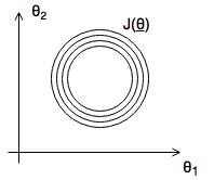
Feature Scaling

Goal: get every feature roughly in the -1..1 range
gradient descent works better / faster when every feature is on the same scale

Example

Unscaled
- $x_1$ : size in ft2 0 – 2000
- $x_2$ : number of bedrooms
Scaled
- $x_1: \frac{\text{size}}{2000} \in [0..1]$
- $x_2: \frac{\#}{5} \in [0..1]$

Mean Normalization

mean value: $\mu_i$
range of values or standard deviation: $S_i$
normalization: $x_i \rightarrow \frac{x_i-\mu_i}{S_i} \qquad\in -0.5\leqslant x_i \leqslant 0.5$

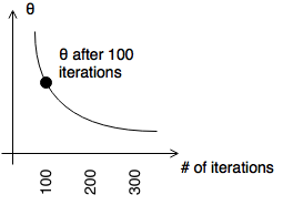
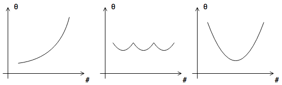
Learning Rate

if \alpha is sufficiently small, J(\overrightarrow{\theta}) decreases on every iteration
need smaller \alpha
\alpha too small

Polynomial Regression

e.g.: cubic model: $\theta_0 + \theta_1 x + \theta_2 x^2 + \theta_3 x^3$

$x$ : size
$x^2$ : size^2
$x^3$ : size^3

Computing Parameters Analytically

Normal Equation solves for $\theta$ analytically (vs. gradient descent is iterative)

$\overrightarrow{\theta}\in\mathbb{R}^{n+1}$
$J(\overrightarrow{\theta}) = J(\theta_0, \theta_1, \cdots, \theta_n) = \frac{1}{2m}\sum^{m}_{i=1}\big(h_{\theta}(x^{(i)}-y^{(i)}\big)^2$
to minimize $J(\overrightarrow{\theta})$
solve for every $j=0..n$
$\frac{\partial}{\partial\theta_j}J(\overrightarrow{\theta})=0$

Parameters are given by $\overrightarrow{\theta} = \big(\underline{X}^T\underline{X} \big)^{-1}\cdot\underline{X}^T\overrightarrow{y}$

where $\underline{X}$ is the feature matrix or design matrix. e.g.:

$x_0$	size $x_1$	bedrooms $x_2$	floors $x_3$	age $x_4$	price $y$
1	2104	5	1	45	460
1	1416	3	2	40	460
1	1534	3	2	30	460
1	852	2	1	36	178

becomes

$\underline{X} = \begin{bmatrix} 1 & 2104 & 5 & 1 & 45 \\ 1 & 1416 & 3 & 2 & 40 \\ 1 & 1534 & 3 & 2 & 30 \\ 1 & 852 & 2 & 1 & 36 \end{bmatrix}_{m\times n+1}$ and $\overrightarrow{y} = \begin{bmatrix} 460 \\ 232 \\ 315 \\ 178 \end{bmatrix}_{m \times 1}$

NB! analytical solution does not require feature scaling
What if X^TX is non-invertible?
- feature matrix has linearly dependent features
  - delete some
- use pseudo-inverse

Gradient Descent in Matrix Form

$m$ samples
$n$ features
$\overrightarrow{\theta}$ parameters $\overrightarrow{\theta} = \begin{bmatrix} \theta_1 \\ \theta_2 \\ \vdots \\ \theta_n \end{bmatrix}_{n \times 1}$
$\overrightarrow{y}$ target $\overrightarrow{y} = \begin{bmatrix} y_1 \\ y_2 \\ \vdots \\ y_m \end{bmatrix}_{m \times 1}$
$\underline{X}$ design matrix or feature matrix $\underline{X} = \begin{bmatrix} x_{11} & x_{12} & \cdots & x_{1n} \\ x_{21} & x_{22} & \cdots & x_{2n} \\ \vdots \\ x_{m1} & x_{m2} & \cdots & x_{mn} \end{bmatrix} = \begin{bmatrix} x^{(1)}_{1} & x^{(1)}_{2} & \cdots & x^{(1)}_{n} \\ x^{(2)}_{1} & x^{(2)}_{2} & \cdots & x^{(2)}_{n} \\ \vdots \\ x^{(m)}_{1} & x^{(m)}_{2} & \cdots & x^{(m)}_{n} \end{bmatrix} = \begin{bmatrix} \overrightarrow{x}^{(1)} \\ \overrightarrow{x}^{(2)} \\ \vdots \\ \overrightarrow{x}^{(m)} \end{bmatrix}_{m \times n}$
$h_{\theta}(\overrightarrow{x})$ hypothesis $\begin{aligned} h_{\theta}(\overrightarrow{x}) & = \theta_1 x_1 + \theta_2 x_2 + \cdots + \theta_n x_n \\ & = \begin{bmatrix} x_1 & x_2 & \cdots & x_n \end{bmatrix}_{1 \times n} \cdot \begin{bmatrix} \theta_1 \\ \theta_2 \\ \vdots \\ \theta_n \end{bmatrix}_{n \times 1} \\ & = \overrightarrow{x}\cdot\overrightarrow{\theta} \end{aligned}$
$J(\overrightarrow{\theta})$ cost function $J(\overrightarrow{\theta}) = \frac{1}{2m}\sum^{m}_{i=1}\big(h_{\theta}(\overrightarrow{x}^{(i)})-y^{(i)}\big)^2$
$\frac{\partial}{\partial\theta_j}J(\overrightarrow{\theta})$ partial derivative of cost function $\begin{aligned} \frac{\partial}{\partial\theta_j}J(\overrightarrow{\theta}) &= \frac{\partial}{\partial\theta_j} \frac{1}{2m}\sum^{m}_{i=1}\big(h_{\theta}(\overrightarrow{x}^{(i)})-y^{(i)}\big)^2 \\ &= \frac{\partial}{\partial\theta_j} \frac{1}{2m}\sum^{m}_{i=1}\big(\overrightarrow{x}^{(i)}\cdot\overrightarrow{\theta} -y^{(i)}\big)^2 \\ &= \frac{1}{2m}\cdot 2 \cdot \sum^{m}_{i=1}\big(\overrightarrow{x}^{(i)}\cdot\overrightarrow{\theta} -y^{(i)}\big) \cdot x_j^{(i)} \end{aligned}$
gradient descent step for a single parameter $\theta_j := \theta_j - \alpha\cdot\frac{\partial}{\partial\theta_j}J(\overrightarrow{\theta})$
gradient descent step $\begin{aligned} \begin{bmatrix} \theta_1 \\ \theta_2 \\ \vdots \\ \theta_n \end{bmatrix} & := \begin{bmatrix} \theta_1 \\ \theta_2 \\ \vdots \\ \theta_n \end{bmatrix} - \alpha\cdot \begin{bmatrix} \frac{\partial}{\partial\theta_1} \frac{1}{2m} \sum^{m}_{i=1}\big(h_{\theta}(\overrightarrow{x}^{(i)}) - y^{(i)}\big)^2 \\ \frac{\partial}{\partial\theta_2} \frac{1}{2m} \sum^{m}_{i=1}\big(h_{\theta}(\overrightarrow{x}^{(i)}) - y^{(i)}\big)^2 \\ \vdots \\ \frac{\partial}{\partial\theta_n} \frac{1}{2m} \sum^{m}_{i=1}\big(h_{\theta}(\overrightarrow{x}^{(i)}) - y^{(i)}\big)^2 \end{bmatrix}_{n \times 1} = \\ \\ & = \begin{bmatrix} \theta_1 \\ \theta_2 \\ \vdots \\ \theta_n \end{bmatrix} - \alpha\cdot \begin{bmatrix} \frac{1}{2m} \cdot 2 \cdot \sum^{m}_{i=1}\big(h_{\theta}(\overrightarrow{x}^{(i)}) - y^{(i)}\big) \cdot x_1^{(i)} \\ \frac{1}{2m} \cdot 2 \cdot \sum^{m}_{i=1}\big(h_{\theta}(\overrightarrow{x}^{(i)}) - y^{(i)}\big) \cdot x_2^{(i)} \\ \vdots \\ \frac{1}{2m} \cdot 2 \cdot \sum^{m}_{i=1}\big(h_{\theta}(\overrightarrow{x}^{(i)}) - y^{(i)}\big) \cdot x_n^{(i)} \end{bmatrix} = \\ \\ & = \begin{bmatrix} \theta_1 \\ \theta_2 \\ \vdots \\ \theta_n \end{bmatrix} - \frac{\alpha}{m}\cdot \begin{bmatrix} \sum^{m}_{i=1}\big(h_{\theta}(\overrightarrow{x}^{(i)}) - y^{(i)}\big) \cdot x_1^{(i)} \\ \sum^{m}_{i=1}\big(h_{\theta}(\overrightarrow{x}^{(i)}) - y^{(i)}\big) \cdot x_2^{(i)} \\ \vdots \\ \sum^{m}_{i=1}\big(h_{\theta}(\overrightarrow{x}^{(i)}) - y^{(i)}\big) \cdot x_n^{(i)} \end{bmatrix} = \\ \\ & = \begin{bmatrix} \theta_1 \\ \theta_2 \\ \vdots \\ \theta_n \end{bmatrix} - \frac{\alpha}{m}\cdot \begin{bmatrix} x_1^{(1)} & x_1^{(2)} & \cdots & x_1^{(m)} \\ x_2^{(1)} & x_2^{(2)} & \cdots & x_2^{(m)} \\ \vdots \\ x_n^{(1)} & x_n^{(2)} & \cdots & x_n^{(m)} \end{bmatrix}_{n \times m} \cdot \begin{bmatrix} h_{\theta}(\overrightarrow{x}^{(1)}) - y^{(1)} \\ h_{\theta}(\overrightarrow{x}^{(2)}) - y^{(2)} \\ \vdots \\ h_{\theta}(\overrightarrow{x}^{(m)}) - y^{(m)} \end{bmatrix}_{m \times 1} = \\ \\ & = \overrightarrow{\theta} - \frac{\alpha}{m}\cdot \underline{X}^T \cdot \Bigg( \begin{bmatrix} \overrightarrow{x}^{(1)} \\ \overrightarrow{x}^{(2)} \\ \vdots \\ \overrightarrow{x}^{(m)} \end{bmatrix}_{m \times n} \cdot \begin{bmatrix} \theta_1 \\ \theta_2 \\ \vdots \\ \theta_n \end{bmatrix}_{n \times 1} - \begin{bmatrix} y_1 \\ y_2 \\ \vdots \\ y_n \end{bmatrix}_{n \times 1} \Bigg) = \\ &= \overrightarrow{\theta} - \frac{\alpha}{m} \cdot \underline{X}^T \cdot \big( \underline{X} \cdot \overrightarrow{\theta} - \overrightarrow{y} \big) \end{aligned}$

Under– and Overfitting

Overfitting: if we have too many features, the learned hypothesis may fit the training set well

$J(\overrightarrow{\theta}) = \frac{1}{2m}\sum^{m}_{i=1}\big(h_{\theta}(x^{(i)})-y^{(i)}\big)^2 \approx 0$

but fails to generalize to new examples

Examples

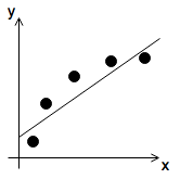
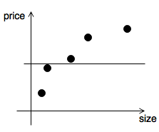
underfit or high bias
- $\theta_0 + \theta_1 x$
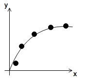
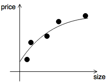
just right
- $\theta_0 + \theta_1 x + \theta_2 x^2$
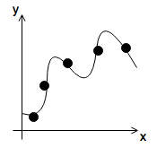
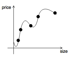
overfit or high variance
- $\theta_0 + \theta_1 x + \theta_2 x^2 \theta_3 x^3 + \theta_4 x^4$

Regularization

To address overfitting one can

reduce number of features
- manually select features to discard
- or employ a model selection algorithm
or add regularization
- keep all of the features of the model
- reduce the magnitude of parameters $\theta_j$
- works well when lot of features are available so that each contributes a little to predicting the value of $y$

Intuition

In the example if we penalize $\theta_3$ and $\theta_4$ and make them small, e.g.: $\min_{\theta} \frac{1}{2m}\sum^{m}_{i=1}\big(h_{\theta}(x^{(i)} - y^{(i)})\big)^2 + 1000\cdot\theta^2_3 + 1000\cdot\theta^2_4$ Smoothes the hypothesis making it fit the training set less, but allows it to generalize better.

Regularization Parameter

Assign small values to every parameter (not just the higher order ones, as demonstrated for the intuition), i.e.: $\theta_0, \theta_1, \cdots, \theta_n$

more simple hypothesis
less prone to overfitting

Housing Example

feautres: $x_0, x_1, \cdots, x_{100}$
$x_0=1$
parameters: $\theta_0, \theta_1, \cdots, \theta_{100}$
cost function with regularization $J(\overrightarrow{\theta})=\frac{1}{2m}\Big[\sum^{m}_{i=1}h_{\theta}(\overrightarrow{x}^{(i)} - y^{(i)})^2 + \lambda\cdot\sum^{n}_{j=1}\theta_{j}^2\Big]$
regularizing term is addded for $\theta_1 \cdots \theta_{100}$ , but not for $\theta_0$
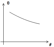
without / too little regularization
- if $\lambda = 0$ , regularization has no effect
\lambda chosen too big
- regularization dominates cost
\lambda chosen just right

Gradient Descent Step

$\begin{aligned} \theta_j & := \theta_j - \alpha\cdot\frac{\partial}{\partial\theta_j}J(\overrightarrow{\theta}) \\ \\ \theta_j & := \theta_j - \alpha\cdot \Bigg[ \frac{1}{m}\sum^{m}_{i=1}\big(h_{\theta}(x^{(i)})-y^{(i)}\big)\cdot x_j^{(i)} + \frac{\lambda}{m}\theta_j \Bigg] \qquad & \begin{aligned} j & = 1,2,\cdots,n\\ j & \neq 0 \end{aligned}\\ \\ \theta_j & := \theta_j \big( 1-\alpha\frac{\lambda}{m} \big) - \frac{\alpha}{m}\sum^{m}_{i=1}\big( h_{\theta}(x^{(i)})-y^{(i)} \big) x_j^{(i)} & 1-\alpha\frac{\lambda}{m} < 1 \end{aligned}$

Normal Equation

feature matrix $\underline{X}= \begin{bmatrix} \overrightarrow{x}^{(1)} \\ \overrightarrow{x}^{(2)} \\ \vdots \\ \overrightarrow{x}^{(m)} \end{bmatrix}_{m \times n+1}$
target $\overrightarrow{y}= \begin{bmatrix} y^{(1)} \\ y^{(2)} \\ \vdots \\ y^{(m)} \end{bmatrix}_{n \times 1}$
goal is to minimize cost function $\frac{\partial}{\partial\theta_j}J(\overrightarrow{\theta}) = 0$
parameters are given by $\theta=\Bigg( \underline{X}^T\cdot\underline{X} + \lambda\cdot \begin{bmatrix} 0 & & & 0 \\ & 1 & & \\ & & \ddots & \\ 0 & & & 1 \end{bmatrix}_{n+1 \times n+1} \Bigg)^{-1} \cdot \underline{X}^T y$
it can be shown, that for $\lambda > 0$ , matrix is always invertible